Isolating_singularities
Motivated by the problem of certified drawing of plane curves, this software is a Python implementation of the algorithms presented in [1]. It basically concerns isolating the singularities of the plane projection of a generic curve embedded in . This type of curves appears naturally in robotics applications and visualization. We present in [1, Section 6] some experiments, some of which are not reachable by other methods. The software can be dowloaded from its GitHub page.
Main functions
In the following, by an interval we mean a list of floats that represent the lower and upper bounds respectively. By a box we mean a list of intervals.
1) enclosing_boxes(system , Box , X , eps_min=0.001,eps_max=0.1)
This function returns a list of two lists: The first one is a list of boxes in that cover a smooth part of the curve (more precisely, where the used solver IbexSolve succeeds to certify the smoothness). The second one contains boxes where the used solver (IbexSolve) fails to certify the smoothness of the curve.
Parameters
system
A string that is the name of the txt file which contains the equations that define the curve.
Box
A box that contains the curve
X
A list of the sympy symbols that appear in the equations of system.
eps_min
Minimal width of output boxes. This is a criterion to stop bisection: a non-validated box will not be larger than ‘eps-min’. Default value is 1e-3.
eps_max
Maximal width of output boxes. This is a criterion to force bisection: a validated box will not be larger than ‘eps-max’ (unless there is no equality and it is fully inside inequalities). Default value is 1e-1.
Example
import Isolating_singularities as isos
import sympy as sp


##################################
#Creating the system file #######
##################################
#The user can creat the txt file manualy where every
#line represents an equation that defines the curve.
#However, the following code is to creat the system
#file using Python.

fil=open("system.txt","w")
fil.write("(x1 - 8*cos(x3))^2 + (x2 - 8*sin(x3) )^2 - 23 \n")
fil.write("(x1 - 9 - 5* cos(x4) )^2 + (x2 - 5* sin(x4))^2 - 60 \n")
fil.write( "(2*x1 - 16*cos(x3))*(2*x2 - 10*sin(x4)) - (2*x2 - 16*sin(x3))*(2*x1 - 10*cos(x4) - 18)")
fil.close()
##################################
#Declaring parameters #######
##################################
System="system.txt"
Box=[[-5,15],[-15,15],[-3.14,3.14],[-3.14,3.14]]
X=[sp.Symbol("x"+str(i)) for i in range(1,5)]

##################################
#Applying the function #######
##################################
boxes =isos.enclosing_curve(System,Box,X)
print(len(boxes[0])) #the number of certified boxes
print(len(boxes[1])) #the number of unknown boxes
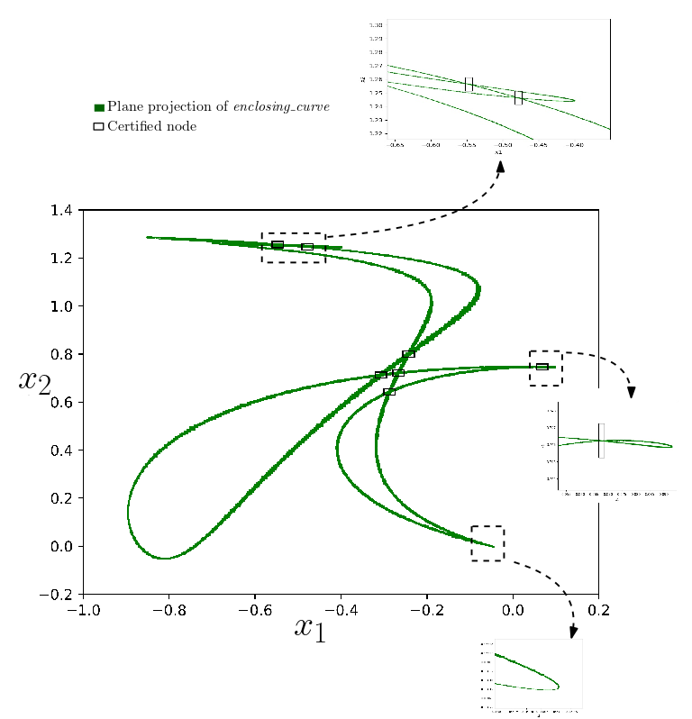
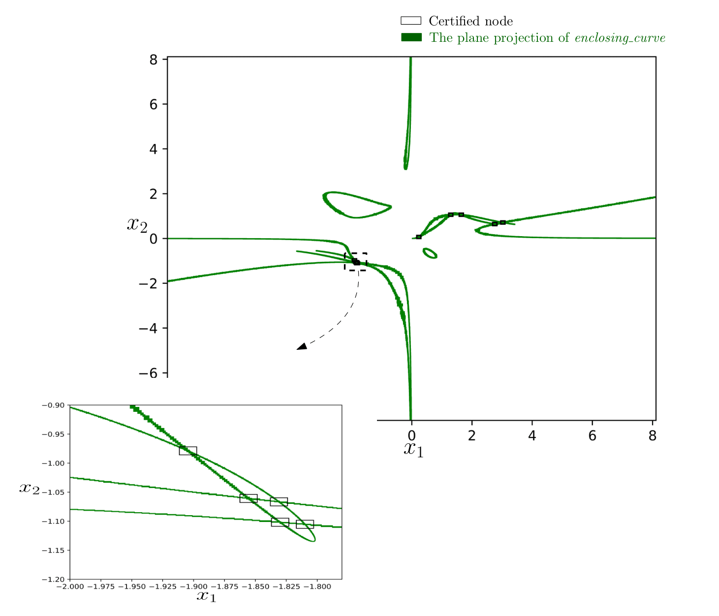
ploting_boxes(certified_boxes, uncer_boxes, var=[0,1], B=[ [-20,20] , [-20,20] ], a=1, b=10, nodes= [], cusps=[ ] )
This function plots a plane projection of output.
Parameters
certified_boxes
A list of boxes that cover a smooth part of the curve certified by IbexSolve. The function plots the plane projection of this list in green.
uncer_boxes
A list of boxes that cover the part of the curve where IbexSolve fails to certify the smoothness. The function plots the plane projection of this list in red.
var (optional)
A list of two integers that determines the variables for which the plane projection is considered.By default, the function considers the first two variables.
B (optional)
Determines the domain of the graph. By defult, it is set to be .
nodes (optional)
A set of boxes each of which contains a node (to be computed later)
cusps (optional)
A set of boxes each of which contains a cusp (to be computed later)
Example
The plane projection with respect to and .
isos.ploting_boxes(boxes[0],boxes[1])
# boxes if the output of enclosing_curve
The plane projection with respect to and .
isos.ploting_boxes(boxes[0],boxes[1],\
        var=[2,3],B=[[-3.14,3.14],[-3.14,3.14]])
enclosing_singularities (System, boxes , Box , X, eps_min=0.001 , eps_mxa=0.1,threshold =0.01 )
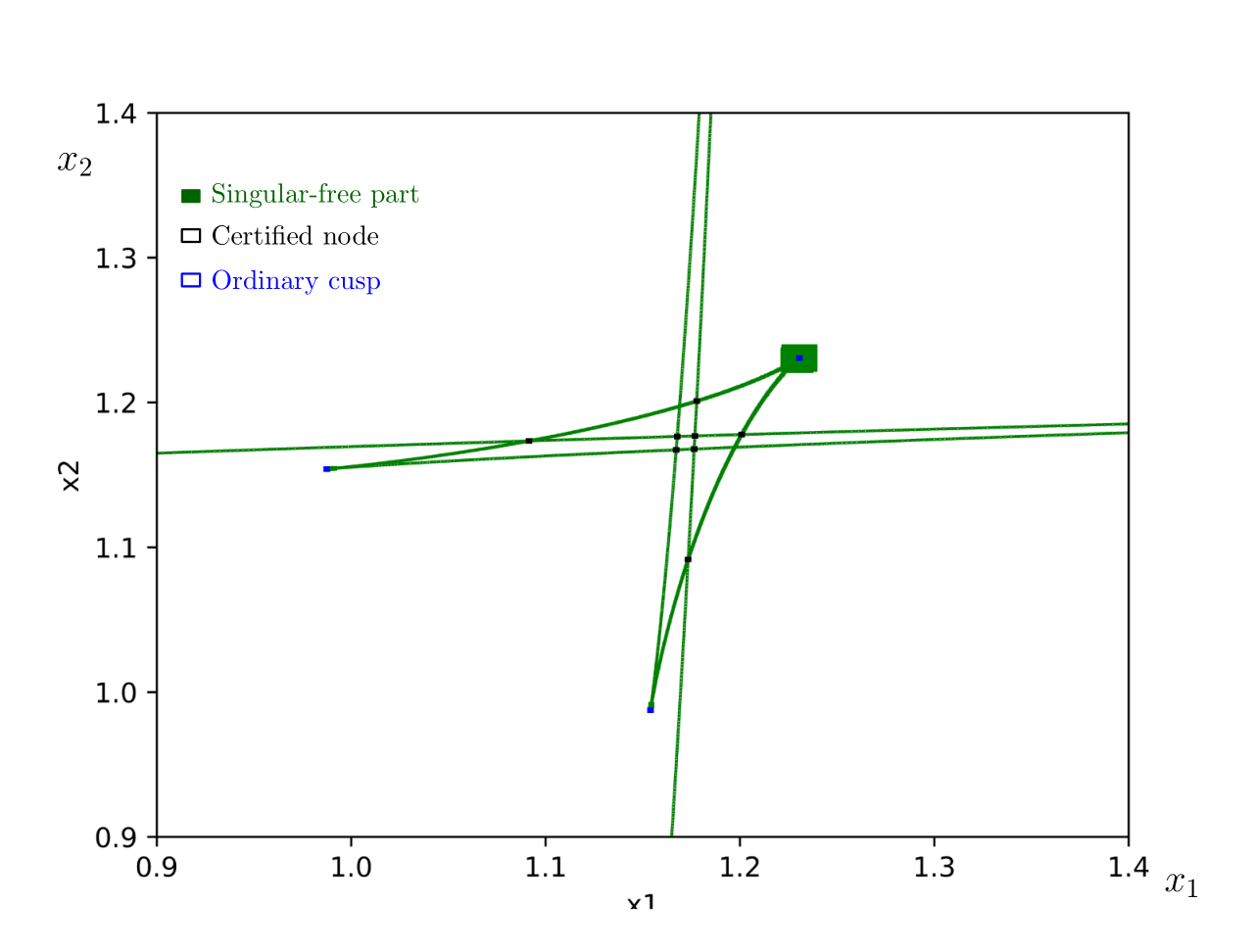
This function returns a set of two sets. The first one contains 2d boxes each of which contains exactly one node of the plane projection (with respect to the first two variables). The second one is a list of boxes such that every box contains either one ordinary cusp or a node that is a projection of two branches closed to each other.
Parameters
System, Box, X, eps_min and eps_max are as in .
boxes is the output of .
threshold A parameter that determines when to use Taylor form instead of the standard way of comuting the Ball system. This improves the performance when there are nodes that are induced by the projection of too-close branches. The default value us 1e-2.
Example
In the following, contains boxes each of which has a solution of Ball with . contains boxes each of which has a solution of Ball with .
nodes, nodes_or_cusps=isos.enclosing_singularities(System,boxes,Box,X)

#plotting the singularities
isos.ploting_boxes(boxes[0],boxes[1],B=[[-5,15],[-15,15]]\
                  ,nodes=nodes, cusps=nodes_or_cusps)
plotting_3D(boxes,Box,var=[0,1,2]):
This function plots the 3D-projection of the given curve with respect to the three variables with the variables indexed by the elements of var. However, the drawing is not certified.
Example
The 3D-projection with respect to the first three variables.
isos.plotting_3D(boxes[0], var=[1,2,3],B=[[-3.14,3.14]*3])
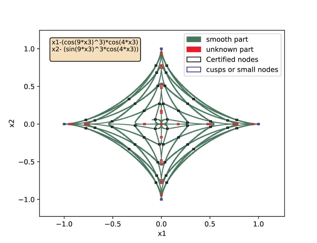
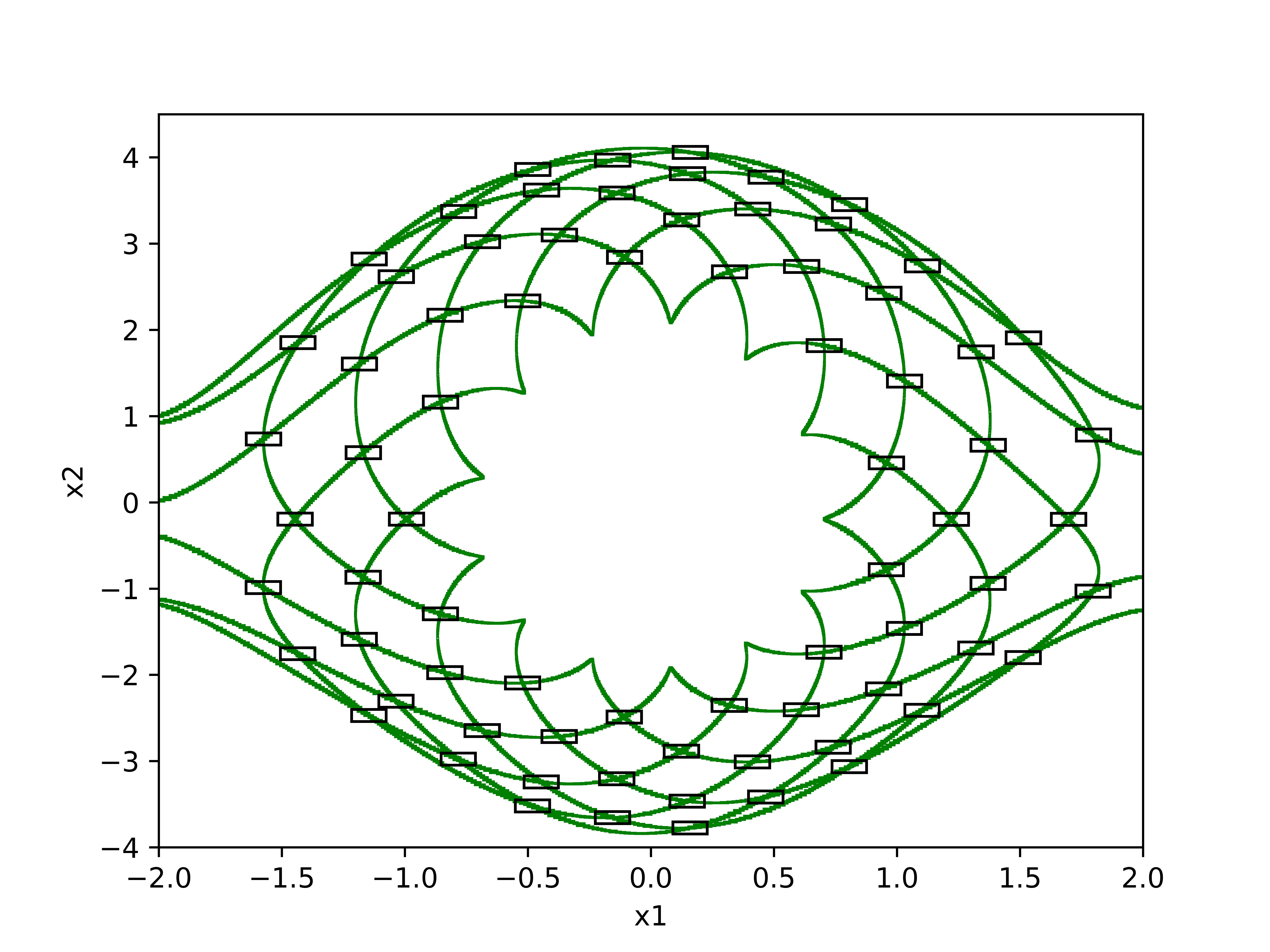
Additional Examples
Here are few additional examples from different types of curves.